Anticipating Critical Alerts in Mining Fleets

The Problem

Mining equipment (haul trucks and excavators) emits a constant stream of telemetry alarms. Among them are the "Don't Go" alerts: conditions in which the equipment must not operate, with a direct impact on safety, fleet availability, and production. The challenge: predict these events hours in advance, turning a historical log into an operational decision tool.

Two obstacles defined the project:

• ·Real scale: tens of millions of telemetry records, processed on a commodity machine, which demanded careful memory engineering.
• ·Rare events:Don't Go alerts are highly imbalanced, which makes accuracy misleading and requires specific metrics and strategies.

The Approach

A reproducible, modular, and tested pipeline covering every stage of a data solution:

• ·Data quality diagnosis and cleaning: identifying and correcting real issues (encoding corruption, null values masked as text, inconsistent decimal separators), with documented change control (before/after + rationale).
• ·Temporal feature engineering: alarm counts across multiple sliding windows, time since the last critical event, and equipment type, all computed in a vectorized way and with no temporal leakage.
• ·Comparative modeling: reference baselines, a main gradient boosting model, and a second approach to cross-validate results, all evaluated on the same temporal split (train on the past, test on the future, never random).
• ·Imbalance handling and a choice of metrics suited to rare events (precision/recall, F1, AUC-ROC, and AUC-PR instead of accuracy).
• ·Explainability and error analysis: SHAP to interpret the model and a critical analysis of where and when it fails (including temporal drift detection).

Results

Don't Go events are rare: only 1.6% of the test window is positive. In that regime a low absolute F1 is the expected outcome, not a failure, and the honest question is not "is F1 high?" but "how much better is this than what operations could do without a model?" So the reference point is the best rule-based heuristic, not a perfect classifier.

Every number in this section comes from the same temporal split: trained on January to April (23,273,520 rows) and tested on May and June (13,890,534 rows), predicting a Don't Go event within the next 4 hours (label_4h), scored at the default decision threshold of 0.5.

• ·XGBoost (selected model), threshold 0.5: F1 0.186, precision 0.111, recall 0.577, AUC-ROC 0.767, AUC-PR 0.205.
• ·Best heuristic baseline (critical_1h > 0): F1 0.038.
• ·Gain: 4.9x the F1 of the best heuristic, and an AUC-PR 12.5x the base rate of the event. Both comparisons are the ones that actually matter operationally.
• ·Cross-check: LightGBM, trained independently as a second approach and scored at the same threshold, landed at F1 0.185. Two different algorithms converging on the same number is evidence that the result comes from the features and the split, not from one lucky model.

Recall was the deliberate priority. Catching 57.7% of the events at 11.1% precision, still at threshold 0.5, means most alerts will not turn into a stop, and that trade is only defensible because the two errors do not cost the same. The next section is where that gets pulled apart.

Error Analysis: Where the Model Breaks

One label before the numbers: the error analysis is run at threshold 0.7, not at the 0.5 used in the section above. The stricter cut buys a little precision for a little recall, landing at recall 0.574 and precision 0.126, with 130,705 true positives, 907,848 false positives, and 96,918 false negatives against 227,623 positive rows. Every count below refers to that 0.7 threshold.

These are row counts, not distinct events. Each telemetry record inside the 4h window before a Don't Go is labelled positive, so a single event contributes many positive rows. Row level is the right unit for scoring the classifier, but converting these figures into a count of anticipated stoppages would require deduplicating by event first.

A model that only reports its wins is not auditable. Breaking those 96,918 false negatives down by month, equipment type, and alarm volume turned out to be the most useful part of the project, because it says precisely where the model can be trusted and where it cannot. The two error types are not interchangeable in the field: a false negative is a Don't Go that was never anticipated, so an unplanned stop, while a false positive is an alert with no Don't Go behind it, so an unnecessary inspection.

• ·Temporal drift: recall is 0.423 in May against 0.922 in June. The same model, on two consecutive months of the same test window, behaves like two different models. Anything shipped on this data needs monitoring and periodic retraining, not a one-off fit.
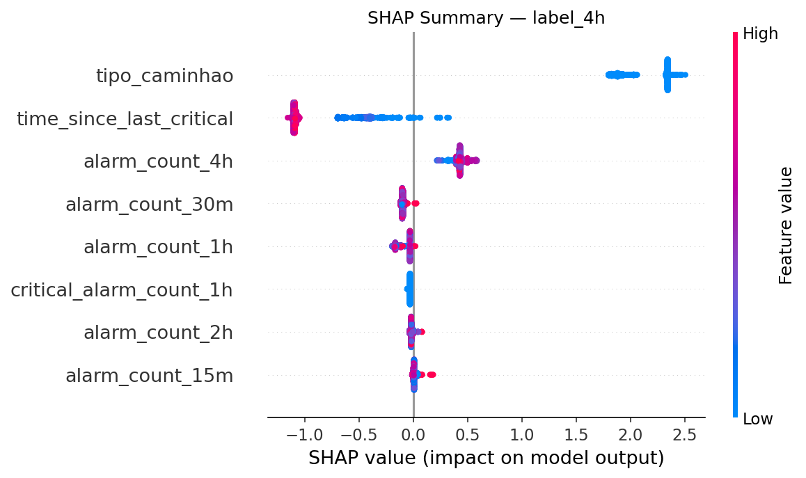
• ·Bias by equipment type: of the 96,918 false negatives, 94,932 are excavators against 1,986 trucks. Almost every miss is an excavator, which lines up with what SHAP had already shown: the model leans on a baseline risk per equipment type instead of on the dynamic alarm pattern.
• ·Concentration in noisy regimes: 96,869 of the 96,918 false negatives sit in the band of 21 or more alarms in 4 hours. Once the equipment is already alarming heavily, the counts saturate and stop discriminating, so the misses pile up exactly where an operator would most want a second opinion.

None of this is solved by moving a threshold. It points at a concrete next iteration: features that separate signal inside high-alarm regimes, and calibration per equipment type rather than a single global model.

Explainability: What the Model Actually Learned

Instead of treating the model as a black box, I used SHAP to understand which signals drive the predictions, and to honestly expose a limitation: the model leans more on a baseline risk per equipment type than on the fine-grained dynamic alarm pattern that precedes a failure. This kind of critical reading is what separates "a model that runs" from "a model that is understood".

Exploratory Analysis: Relationships Between Variables

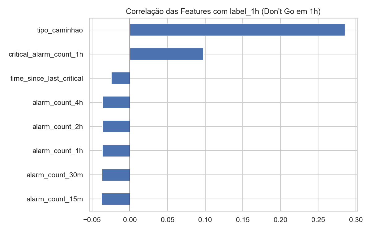
Before modeling, I mapped the structure of the data and the relationships between the engineered features, identifying redundancies (multicollinearity) and hypotheses to test during modeling.

What I Learned

• ·Engineering matters as much as the model. Much of the effort went into making the pipeline viable at real scale (data type and memory optimization), a problem that only shows up outside the toy dataset.
• ·Analytical honesty is a skill.Reporting the model's limitations (bias by equipment type, temporal drift, cost of false positives) is worth more than dressing up a result.
• ·Software rigor in data science. Test-driven development (TDD), documented decisions, and reproducibility turn an exploratory notebook into an auditable solution.

Stack

Skills Demonstrated

Data engineering / ETL at scale · Temporal feature engineering · Machine learning with imbalanced classes · Temporal validation (no data leakage) · Model and baseline comparison · Explainability (SHAP) · Error and drift analysis · TDD and reproducibility · Technical communication and translation into business impact.